“Reality is built in wonderful simplicity”, Eliyahu Goldratt “The Choice”

Scheduling and Resource Allocation are traditionally considered as very complex business problems. They are usually out of reach for the most rule engines.  I personally learned how to deal with these complex problems during my real-world consulting practice by applying a great product called “ILOG Scheduler” written by Claude LePape and Jean-Francois Puget 20 years ago. I’ve just googled the product name and got this User Manual that has over 600 pages with a lot of C++ code. I used to teach ILOG Solver/Scheduler courses and will reuse some examples borrowed from them.

The intention of this post is to follow Eli Goldratt’s principle of “Inherent Simplicity” (“every situation, no matter how complex it initially looks, is exceedingly simple“) and to demonstrate that a business analyst without C++, Java, or any programming background is still capable to do decision modeling even in such complex business domain.

Generic Model

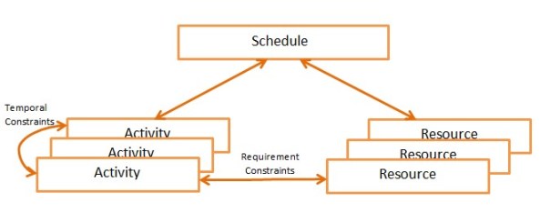
A scheduling and resource allocation problem can be defined in terms of activities and resources as described on the following generic diagram:

The Schedule is defined in time and has origin (start) and horizon (end).  The Schedule usually consists of activities, resources, and different relationships between them. Activities may have known or unknown start, duration and end, and we may assume that there is a natural constraint between them (start + duration = end). There can be precedence relationships between activities such as “Job A start after the end of the job B”. These relationships are usually called “temporal constraints”.

Resources usually have limited capacities may vary over time. For example, a person may be available only certain hours during the day. Resources may have different types:  recoverable like humans or consumable like money or gasoline.  Activities may require or produce different resources, and the proper constraints are usually called “Resource Requirement Constraints”.  There are many implementation details but basically the above high-level schema allows us to do decision modeling for many practical problems.

Example: Schedule Activities

We will start with a very simple example and will add more complexity as we go on. So, let’s assume that we plan to construct a house. The construction requires the following activities with fixed durations and precedence constraints:

Arrows represent temporal constraints like “Carpentry starts after the end of Masonry”. The numbers near each activity represent its durations (in days).

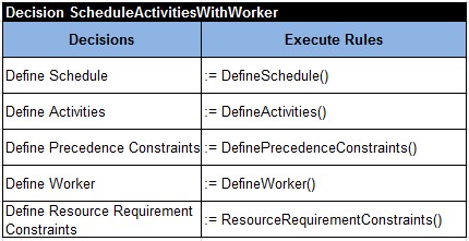
To model this, pure scheduling, problem I will use OpenRules Rule Solver and Excel-based decision tables placed only in one file “Decision.xls”. Our decision “ScheduleActivities” can be defined in the following decision table through 3 sub-decisions:

The first sub-decision simply defines the schedule as:

It simply states that the schedule should be completed in 29 days (a simple sum of all activity durations). Why Schedule’s origin is 0? We always assume that each time interval [start;end) includes left bound and does not include the right bound, e.g. the last day of this schedule is [29;30).

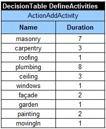
We may define all activities in this decision table:

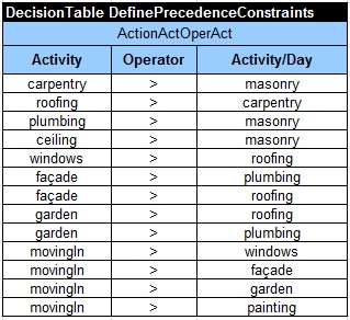
And finally, we define all precedence constraints in this table:

If we run the file Decision.xls with Rule Solver, it will produce the following results:

masonry[0 — 7 –> 7)
carpentry[7 — 3 –> 10)
roofing[10 — 1 –> 11)
plumbing[7 — 8 –> 15)
ceiling[7 — 3 –> 10)
windows[11 — 1 –> 12)
façade[15 — 2 –> 17)
garden[15 — 1 –> 16)
painting[0 — 2 –> 2)
movingIn[17 — 1 –> 18)

Hope the notation is obvious: activity[start — duration –> end).

Example: Schedule Activities with a Worker

Now let’s make our problem a little bit more complex. Let’s assume that all of the activities require a worker in order to be processed. Because the worker can only perform one task at a time, we cannot schedule two activities at the same time (as we could in the basic example).

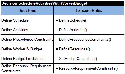
So, we need to add two more sub-decisions to our previous decision as described below:

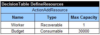
We may define a worker as a recoverable resource with maximal capacity equal to 1 day:

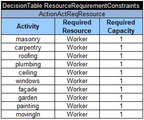
The next decision table states that each activity requires this resource “Worker”:

The extended problem is now defined and we again may execute the file Decision.xls with Rule Solver. Here are new results:

masonry[0 — 7 –> 7) requires Worker[1]
carpentry[7 — 3 –> 10) requires Worker[1]
roofing[10 — 1 –> 11) requires Worker[1]
plumbing[11 — 8 –> 19) requires Worker[1]
ceiling[19 — 3 –> 22) requires Worker[1]
windows[22 — 1 –> 23) requires Worker[1]
façade[23 — 2 –> 25) requires Worker[1]
garden[25 — 1 –> 26) requires Worker[1]
painting[26 — 2 –> 28) requires Worker[1]
movingIn[28 — 1 –> 29) requires Worker[1]

Example: Schedule Activities with a Worker and a limited Budget

Let’s continue adding more complexity to our example. Now along with worker constraints, we have to consider budget constraints. Each activity requires the payment of $1,000 per day. Let’s assume that a bank agreed to finance the house constructions for the total amount of $29,000. However, the sum is available in two installations, $13,000 is available at the start of the project, and $16,000 is available 15 days afterwards. How could we still construct the house under these constraints?

Let’s expand our decision with three more sub-decisions that define a resource “Budget”, set its capacities, and add budget requirement constraints:

We may add a resource “Budget” to the same table that defines “Worker”, but we should keep in mind that budget cannot recover and is being consumed by activities:

As we already specified maximal capacity of the resource budget, it is enough to specify the limit $15,000 for the first 15 days:

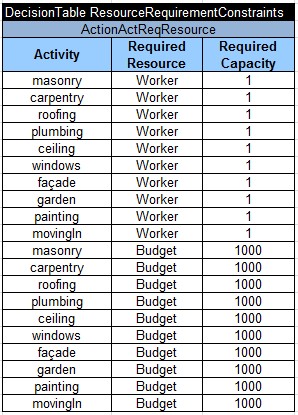
The extended table “ResourceRequirementConstraints” will look as follows:

The modeling part is over and we can again execute the updated file Decision.xls. Here are new results:

masonry[0 — 7 –> 7) requires Worker[1]  requires Budget[1000]
carpentry[7 — 3 –> 10) requires Worker[1]  requires Budget[1000]
roofing[10 — 1 –> 11) requires Worker[1]  requires Budget[1000]
plumbing[11 — 8 –> 19) requires Worker[1]  requires Budget[1000]
ceiling[19 — 3 –> 22) requires Worker[1]  requires Budget[1000]
windows[22 — 1 –> 23) requires Worker[1]  requires Budget[1000]
façade[23 — 2 –> 25) requires Worker[1]  requires Budget[1000]
garden[25 — 1 –> 26) requires Worker[1]  requires Budget[1000]
painting[26 — 2 –> 28) requires Worker[1]  requires Budget[1000]
movingIn[28 — 1 –> 29) requires Worker[1]  requires Budget[1000]

Example: Schedule Activities with Alternative Resources

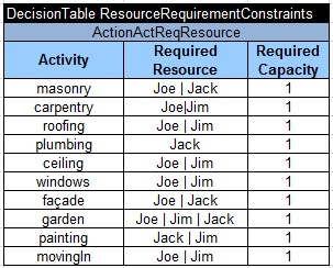
Now let’s consider the initial scheduling problem when jobs can be executed by different workers – alternative resources. Let’s assume that we have three workers Joe, Jim, and Jack, with different skills. Each job requires only one of these workers depending on their skills:

masonry    requires Joe or Jack
carpentry  requires Joe or Jim
plumbing   requires Jack
ceiling        requires Joe or Jim
roofing       requires Joe or Jim
painting     requires Jack or Jim
windows    requires Joe or Jim
façade        requires Joe or Jack
garden       requires Joe or Jack or Jim
movingIn   requires Joe or Jim.

We may extend the Decision with two more sub-decisions:

The sub-decision “DefineWorkers” adds 3 alternative resources that should be specified as special “disjunctive” resources:

The next decision table is similar to previous “ResourceRequirementConstraint” tables but lists different alternative resources separated by the or-sign “|”:

This completes the modeling and after the execution of the modified file “Decision.xls” our Rule Solver will produces new results telling exactly “who does what”:

masonry[0 — 7 –> 7) requires Jack[1]
carpentry[7 — 3 –> 10) requires Jim[1]
roofing[10 — 1 –> 11) requires Jim[1]
plumbing[7 — 8 –> 15) requires Jack[1]
ceiling[7 — 3 –> 10) requires Joe[1]
windows[11 — 1 –> 12) requires Jim[1]
façade[15 — 2 –> 17) requires Jack[1]
garden[15 — 1 –> 16) requires Jim[1]
painting[0 — 2 –> 2) requires Jim[1]
movingIn[17 — 1 –> 18) requires Jim[1]

How Rule Solver Works

Rule Solver reads an Excel-based decision model and “on the fly” generates the proper constraint satisfaction problem using the standard Constraint Programming API “JSR-331”. Then it validates and solves the problem using one of several available constraint solvers that are JSR-331 compliant. Being based on the JSR-331, Rule Solver allows you to switch between different underlying CP solvers without any changes in the decision model. Those CP solvers are very powerful tools that utilize the results of the last 25 years R&D done by CP experts around the globe.  While internal implementations of the resource requirement constraints  and search strategies can be extremely complex, the modeling facilities of Rule Solver remain simple, intuitive, extendable, and oriented to business analysts (not to programmers or CP gurus). 

Conclusion

Described decision models demonstrate that even complex scheduling and resource allocation problems can be modeled relatively easy without programming. Note that our decision models only define problems and do not tell anything how to resolve them. Concentrating on “WHAT” and ignoring “HOW” is a natural approach for a modeling environment such as OpenRules Rule Solver that is oriented rather on subject matter experts than on software developers. At the same time, Rule Solver provides a special Java API to do similar modeling in Java or mix&match both approaches.  You may learn more about modeling and solving these and other constraint satisfaction problems with the latest version of the Rule Solver that will become available early on March 2012 in the upcoming Release 6.2.0 of OpenRules BDMS.